I ran an experiment two days ago. Two architectures, but same task and model.

A code review, refactor, and test suite for a 20-line Python function. First, I gave it to one LLM call. Do everything in a single response. Then I split it across three agents: a reviewer, a refactorer, and a test writer. Each agent received the previous agent’s output and built on it.

Same model. Same task. Comparable output quality.

The multi-agent pipeline consumed 2.4x more tokens.

Not 20% more. Not 50% more. 2.4 times. 44,789 tokens versus 18,395. The three-agent version also took 30% longer wall-clock time, made 3 separate API calls, and produced output that was, by any reasonable measure, about the same quality as the single call.

I build multi-agent systems. I use them daily. And I had never once looked inside the machine to understand why the bill was what it was.

This article is what I found when I did.

Every Token Is a Prediction That Depends on Every Previous Token

Most developers don’t realize this about LLM inference: it’s sequential.

When you send a prompt to Claude or GPT, the model doesn’t generate the entire response at once. It generates one token at a time, left to right, and each token depends on every token that came before it.

Input:  "Write a function that sorts a list"

Step 1: Model sees input → predicts "def"
Step 2: Model sees input + "def" → predicts "sort"
Step 3: Model sees input + "def sort" → predicts "_list"
Step 4: Model sees input + "def sort_list" → predicts "("
...repeat for every token in the response

This is called autoregressive generation. The “auto” part means each output feeds back as input for the next step. The model doesn’t plan ahead. It doesn’t outline the response and then fill it in. It commits to each token before it knows what the next one will be.

For a 1,000-token response, that’s 1,000 sequential prediction steps. Each step attends to every previous token. Naively, this scales quadratically with sequence length. Modern architectures optimize this closer to linear, but the sequential dependency remains. You can’t parallelize token 500 until tokens 1 through 499 exist.

Generating long responses is inherently slow. Not because the GPU is weak. Because the algorithm waits.

This is why streaming exists. The model isn’t waiting to finish and then sending you the result. It literally doesn’t know what the full result is until it generates the last token.

The KV Cache: The Memory Structure That Eats Your GPU

This is where it gets expensive.

At each generation step, the model computes “attention” over all previous tokens. Attention is how the model decides which earlier tokens matter for predicting the next one. When it encounters “it” in a sentence, it attends to earlier nouns to figure out what “it” refers to.

Without caching, every new token means re-processing the entire sequence. Token 10,001 in a conversation? Re-compute attention over all 10,000 previous tokens. Token 10,002? All 10,001. That’s quadratic cost per token.

The solution is the KV cache (Key-Value cache). During each attention computation, the model produces two vectors for each token: a Key and a Value. Instead of throwing these away, the system stores them. When the next token is generated, the model only needs to compute the Key and Value for the new token, then look up the cached Keys and Values for all previous tokens.

Without KV cache:
  Token 1000: compute attention over tokens 1-999 (999 operations)
  Token 1001: compute attention over tokens 1-1000 (1000 operations)
  Token 1002: compute attention over tokens 1-1001 (1001 operations)

With KV cache:
  Token 1000: compute K,V for token 1000, attend to cached K,V for 1-999
  Token 1001: compute K,V for token 1001, attend to cached K,V for 1-1000
  Token 1002: compute K,V for token 1002, attend to cached K,V for 1-1001
  (cached values are reused, not recomputed)

The tradeoff: memory. The KV cache grows linearly with sequence length. For a model like Llama 4 Maverick (17B active parameters, 128 experts) running on an NVIDIA B200, the KV cache for a long sequence consumes serious GPU memory even on hardware with 180 GB of HBM3e. At the 10M token context window that Llama 4 Scout supports, the cache dwarfs the model weights.

To make this concrete, take a simpler example. A 70B-class dense model with 80 layers, 8 KV heads, and 128-dim heads at BF16 precision:

KV cache size = 2 × num_layers × head_dim × num_kv_heads × seq_length × bytes

At 128K tokens (BF16):
= 2 × 80 × 128 × 8 × 128,000 × 2 bytes
≈ 41 GB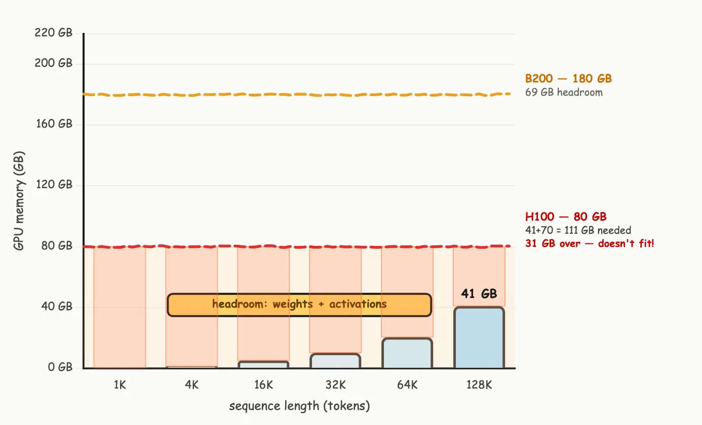

41 gigabytes. For the cache alone. Not the model weights. Not the activations. Just the stored Keys and Values from previous tokens. On an older A100 (80 GB), that’s half the GPU gone. Even on a B200 (180 GB), it’s a serious chunk once you account for model weights and activation memory.

At long context, you’re spending more GPU memory remembering what you said than thinking about what to say next. This is why long-context inference is expensive even when the model architecture supports it. The context window is a memory problem disguised as a feature.

Continuous Batching: Your Request Is Not Alone

When you send a request to an LLM API, your prompt doesn’t get exclusive access to a GPU. It enters a queue alongside hundreds or thousands of other requests.

Modern serving frameworks like vLLM and TensorRT-LLM use continuous batching: at every generation step, the system checks whether any request has finished, evicts it, and inserts a new one. The GPU stays full. No wasted cycles.

Why this matters for your agents: each hop enters the queue independently. Agent 2 can’t start until Agent 1’s response is fully generated and returned to your application. Your three agents don’t run on the same GPU in sequence. They queue, wait, run, return, queue, wait, run, return.

What Happens When You Stack Agents

Now apply everything above to a multi-agent pipeline.

I ran a task through three agents: a code reviewer, a refactorer, and a test writer. This is what actually happened at the inference level:

Agent 1 (Reviewer):
Receives the code snippet (the original prompt). Builds a KV cache for the input tokens. Generates the review autoregressively, token by token. Total: 13,056 tokens consumed. KV cache built and then discarded when the request completes.

Agent 2 (Refactorer):
Receives the original code snippet PLUS Agent 1’s entire review output. Builds a brand new KV cache from scratch. The model re-encodes the original code (already processed by Agent 1) and re-encodes the review (already generated by Agent 1). Total: 13,328 tokens consumed. KV cache discarded.

Agent 3 (Test Writer):
Receives Agent 2’s refactored code (which implicitly contains the decisions from Agent 1’s review). Builds yet another KV cache from scratch. Total: 18,405 tokens consumed. KV cache discarded.

There is no shared KV cache between agent hops. Agent 2 cannot peek into Agent 1’s cached Keys and Values. Each agent starts from a cold cache, re-processes all the context it was given, and then discards everything when it’s done.

The mental model of “agents collaborating” maps to the reality of “three strangers reading the same document in sequence and writing memos to each other.” Each stranger starts from page one.

The Optimizations That Try to Cheat Physics

The inference stack has several tricks to reduce these costs. None of them eliminate the core problem, but they change the math considerably.

Speculative Decoding

The bottleneck in autoregressive generation is that each token is generated sequentially. Speculative decoding, now widely adopted in production and built into frameworks like vLLM, uses a smaller, faster “draft” model to guess multiple tokens at once, then the larger model verifies those guesses in parallel.

Normal autoregressive (5 tokens):
  Big model: predict T1 → predict T2 → predict T3 → predict T4 → predict T5
  (5 sequential steps)

Speculative decoding (5 tokens):
  Small model: quickly guess T1, T2, T3, T4, T5
  Big model: verify all 5 in one parallel forward pass
  Accept: T1 ✓, T2 ✓, T3 ✓, T4 ✗ → keep T1-T3, regenerate from T4
  (2 steps instead of 5, if acceptance rate is high)

The speedup depends on the acceptance rate, which is how often the draft model’s guesses match what the big model would have generated. The original speculative sampling paper demonstrated 2–2.5x decoding speedups. Production implementations with well-matched draft models can push beyond that, depending on the task and acceptance rate.

The catch: speculative decoding doesn’t reduce the total compute. It increases GPU utilization by doing more work in parallel. The draft model consumes its own compute, and rejected tokens are wasted work. It trades compute efficiency for latency reduction.

Quantization

Full-precision LLMs typically use BF16 (bfloat16) for each parameter. A 70B parameter model at BF16 requires 140 GB of memory just for the weights. That fits on a single B200 (180 GB) but not on an H100 (80 GB).

Quantization shrinks those weights. The state of play in 2026: FP8 is the new default on Blackwell GPUs, with native hardware support via the 2nd-gen Transformer Engine. INT8 and INT4 still dominate on older hardware. GPTQ and AWQ remain the go-to post-training methods, with FP8 and GGUF growing alongside them.

70B dense model memory requirements:
  BF16:  140 GB  (fits on 1x B200 180GB)
  FP8:    70 GB  (fits on 1x H100 80GB)
  INT4:   35 GB  (fits on workstation GPUs like A6000 48GB)

The tradeoff is quality. FP8 and INT8 quantization show what the GPTQ paper calls “negligible accuracy degradation” on most benchmarks, though the exact impact varies by model and task. INT4 is more aggressive: depending on the task, the quality gap becomes noticeable. For many application-level tasks, the difference is undetectable. For complex reasoning or code generation, it can matter.

The relevance for multi-agent systems: if your coordination agent (the one routing tasks to specialists) doesn’t need the full model’s reasoning capability, running it on a quantized smaller model can cut your per-hop costs considerably. The review agent might need FP8 precision. The router might be fine at INT4.

One more optimization worth mentioning: prefix caching. Providers like Anthropic and OpenAI offer cheaper rates for cached input tokens when prompts share a common prefix (like a system prompt). This helps if your agents share the same system prompt, but it does nothing for the context duplication problem. Each agent’s input is different because it includes the previous agent’s output. The part that’s expensive is exactly the part that can’t be cached.

What This Means for Your Architecture

The 2.4x overhead I measured is for a simple three-agent chain. Real multi-agent systems are worse.

Consider a “team of agents” pattern where a planner agent routes to three specialist agents, then an aggregator agent synthesizes their outputs. That’s five hops. Each hop re-encodes its full input. The planner’s context is duplicated into every specialist. Every specialist’s output is duplicated into the aggregator. The token multiplication is not additive. It’s combinatorial.

Planner → Specialist A → ┐
        → Specialist B → ├→ Aggregator → Output
        → Specialist C → ┘

Hops: 5 (planner + 3 specialists + aggregator)
Context duplication: planner's output is in 3 specialist inputs
                     + all 3 specialist outputs are in aggregator input

Before you add another agent to your pipeline, do this math:

1. Count the hops. Each hop is a full inference call with its own KV cache.
2. Measure the context growth. How many tokens does each agent receive? How much of that is duplicated from a previous agent?
3. Ask: could a single call do this? The single call costs 1x. Three agents cost 2.4x. Five agents will cost more. At some point, a longer prompt to one model is cheaper than a shorter prompt to five.
4. Quantize the coordinator. If you must use agents, run the routing/planning agent on a smaller or quantized model. Save the big model for the agents doing the actual reasoning.
5. Measure your prefix cache hit rate. If your agents share system prompts, you’re getting some savings. If every agent has a unique prompt, you’re paying full price on every hop.

The abstraction of “a team of AI agents” is useful for thinking about problem decomposition. It’s misleading for thinking about cost. The GPU doesn’t see a team. It sees sequential batch jobs with no shared memory, each one re-reading everything the last one already processed.

I looked at my own pipeline after running this experiment. Five agents. I’d been paying for five cold starts on every task and calling it orchestration.

Open your API dashboard. Count the hops. Do the math. The abstraction was never hiding complexity from you. It was hiding the invoice.

—Viz